Polynomial functions are algebraic functions in which the mathematical expression is a polynomial - terms consisting of coefficients and variables that are added or subtracted together.
We can observe a fascinating property when we create a table of values for polynomial functions and evaluate their differences. Let's consider two functions:
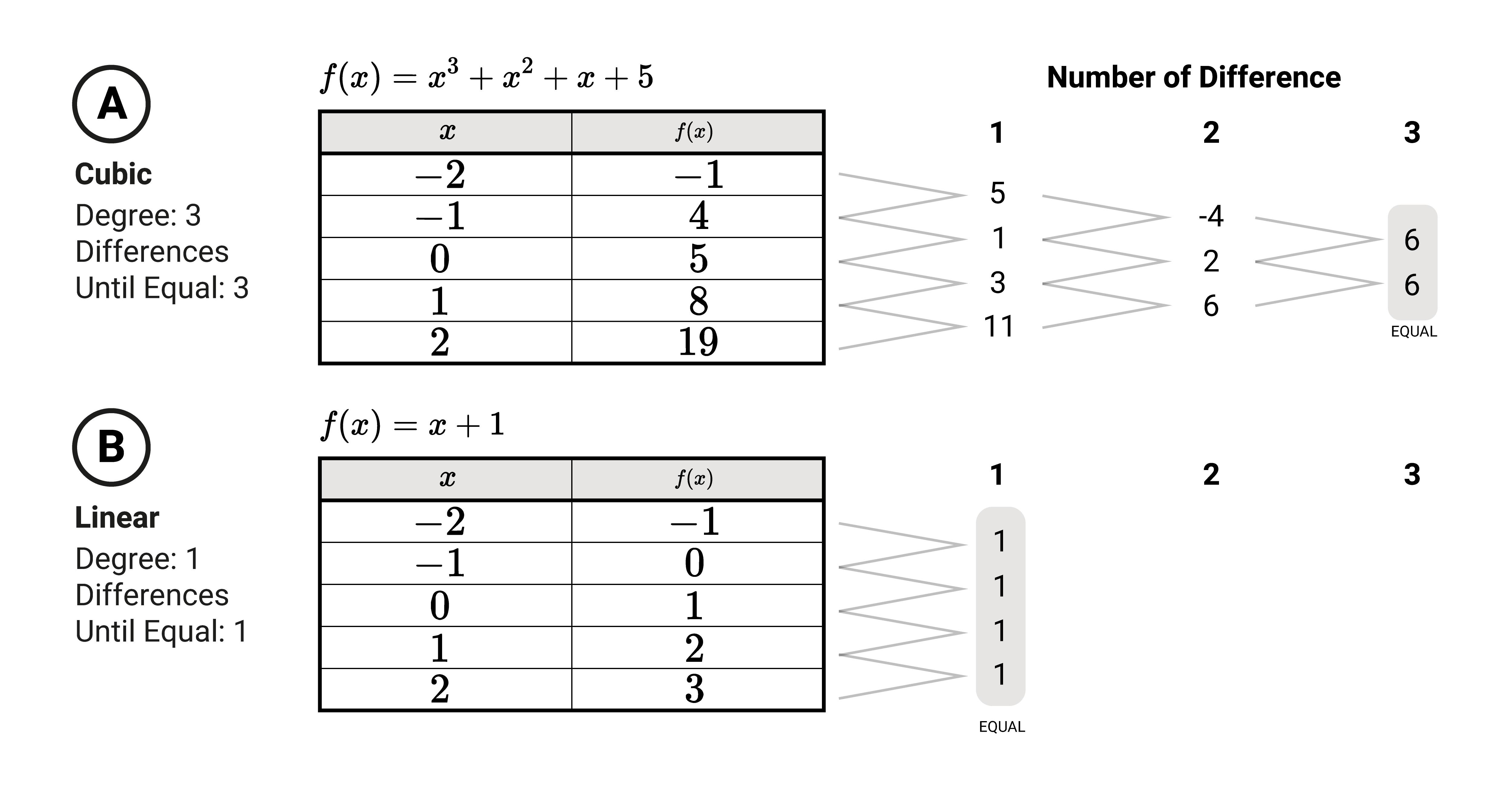
\(f(x)=x^3+x^2+x+5\) - a cubic function (degree 3)
\(f(x)=x+1\) - a linear function (degree 1)
Let's create a table of values for each and try evaluating the outputs given -2, -1, 0, 1, and 2 as inputs. Afterward, we take the difference between adjacent output values until we reach a point where the differences are the same.
Observe that:
For the cubic function, it will take you three differences
For a linear function, it will only take you one difference
The number of times we must take the difference between adjacent values to reach a common difference equals the polynomial degree of the function.
Graphical Perspective
Polynomial functions have interesting graphical properties. Below is a table of \(n\) polynomial functions with their graphs. Here are some notable illustrations one can take off when analyzing their plots:
The graph of a constant function is a horizontal line
The graph of a linear function is a line
The graph of a quadratic function is a parabola
Constant (n=0)
Linear (n=1)
Quadratic (n=2)
Cubic (n=3)
Quartic (n=4)
Transformations
We can make different transformations to the graphs of polynomial functions. For example, we can move it or create a mirror of it. The following section shows how we apply these transformations.
Let's consider a quadratic function: \(f(x)=x^2\). The graph is a parabola with its vertex at the origin \((0,0)\)
Translation
Horizontal
Translation (Horizontal)
Say we want to translate our quadratic function to the left or right. We introduce a constant \(c\) to the input \(f(x±c)\) to accomplish this.
The graph moves to the right if \(c\) is negative.
It moves to the left if \(c\) is positive.
Let's move our graph example one unit horizontally. The possible expressions would be the following:
If we have \(f(x)=(x+1)^2\), the graph will translate three units to the left.
If we have \(f(x)=(x-1)^2\), it will translate three units to the right.
Vertical
Translation (Vertical)
Let's consider the translation of our graph in up or down directions. Again, we introduce a constant \(c\) that we will add to the polynomial function: \(f(x)±c\)
The graph moves upward if \(c\) is positive.
It moves downward if \(c\) is negative.
Let's move our graph example one unit vertically. The possible expressions would be the following:
If we have \(f(x)=(x)^2+1\), the graph will translate three units upward.
If we have \(f(x)=(x)^2-1\), it will translate three units downward.
From this \(c\), we can make an additional observation: the constant term of the polynomial function dictates the vertical movement of the graph.
Reflection
Reflection
Reflection deals with a graph's mirror transformation (or symmetry) about a particular line. We consider the signs to investigate this transformation.
\(f(-x)\) will reflect the graph about the y-axis.
\(-f(x)\) will reflect the graph about the x-axis.
\(-f(-x)\) will reflect the graph about the origin.
To have a better view, let's consider another function, \(f\left(x\right)=x^{3}+x^{4}\). The following are the possible reflection transformations of the graph:
If we have \(f\left(x\right)=\left(-x\right)^{3}+\left(-x\right)^{4}\), we will reflect the graph about the y-axis. See \(g(x)\)
If we have \(f\left(x\right)=-\left(x^{3}+x^{4}\right)\), we will reflect the graph about the x-axis. See \(h(x)\)
If we have \(f\left(x\right)=-\left(\left(-x\right)^{3}+\left(-x\right)^{4}\right)\), we will reflect the graph about the origin. See \(i(x)\)
These are some sample transformation methods we use to modify the graph of a function. We can combine different transformations to create plots that would suit our needs.
Summary
If a polynomial is in terms of a function, it is a polynomial function.
We can express the general form of a polynomial function as: \(f(x)=a_n x^n+a_{n-1} x^{n-1}+\cdots+a_2 x^2+a_1 x+a_0\)
When dealing with such functions, we usually define them by the degree of the polynomial \(n\).
Numerically speaking, the number of times we must take the difference between adjacent outputs to reach a common difference equals the polynomial degree \(n\).
Polynomial functions have interesting graphical properties. For example, the graph of a constant function is a horizontal line, a linear function is a line, and a quadratic function is a parabola.
We can make different transformations to the graphs of polynomial functions, such as translation or reflection.