
Another application of differential equations (DE) is modeling growth or decay events with a limit. This post explains more about this event:
Modeling Logistics
Let's recall that for some phenomena, the rate of change is directly proportional to its quantity, just like we did with growth and decay; However, this is only sometimes the case. To illustrate, let's look at population growth. We can model it exponentially as \(y=Ce^{kt}\), but this assumes that the population will grow infinitely.
As time passes, population growth decreases because of a specific limitation \(L\). It happens due to a lot of factors. In our example, the growth slowed down probably because the place has limited resources to offer its people; hence, people leave the area. As a consequence, it regulates growth.
It may be best to model these events using the logistic differential equation. Pierre François Verhulst, a Belgian Mathematician, first created this equation. It states that the rate of change is directly proportional to the difference between quantity \(y\) and a limiting term \(\frac{y^2}{L}\):
- \(\frac{d y}{d t} \propto \left(y-\frac{y^2}{L}\right)\)
- \(\frac{d y}{d t} \propto y\left(1-\frac{y}{L}\right)\)
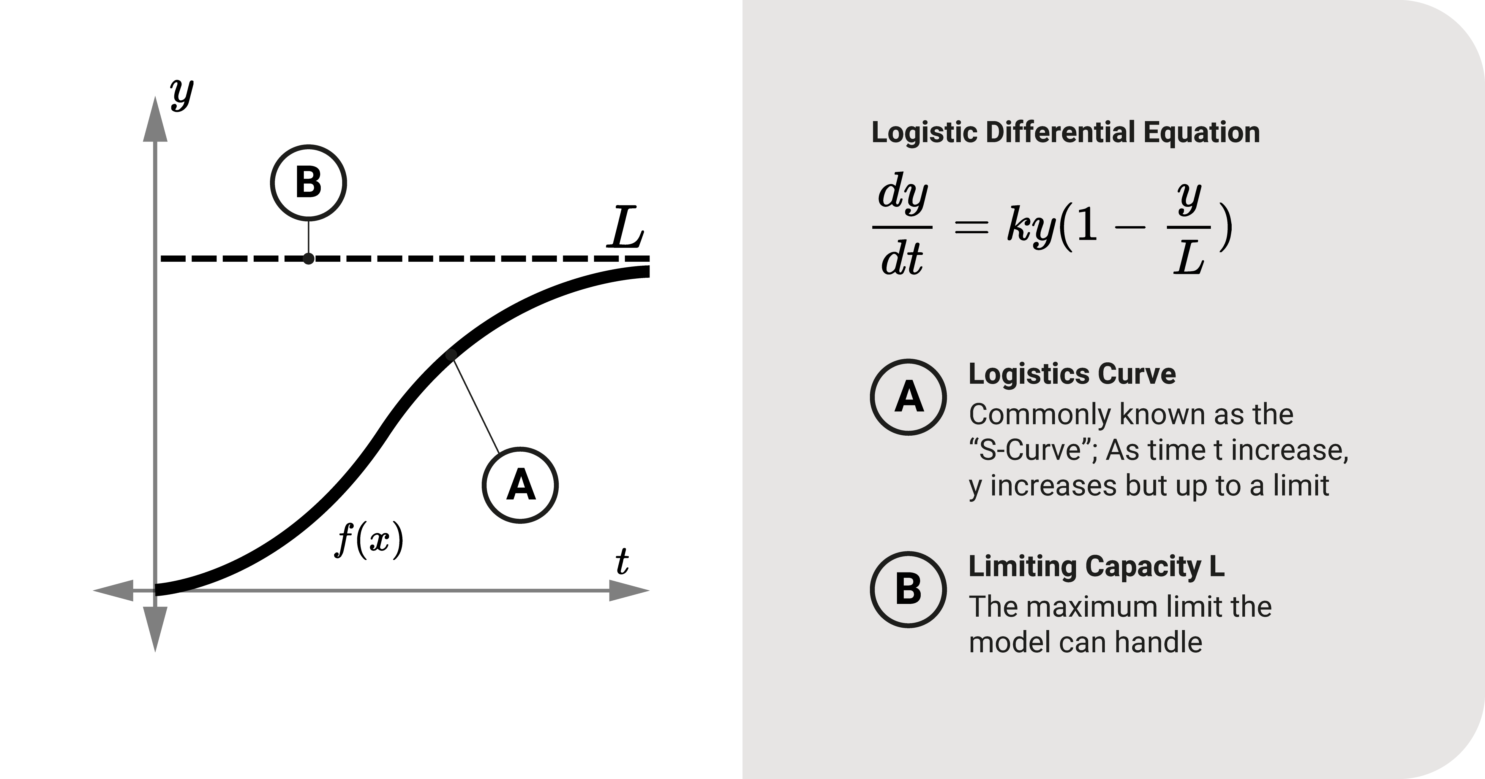
- \(\frac{d y}{d t}=k y\left(1-\frac{y}{L}\right)\)
The model grows at a \(k\) growth rate as time \(t\) goes by. At some point, \(y\) would approach a limiting capacity \(L\).
We can find the general solution using the separation of variables method or Bernoulli's Equation. Let's use the latter:
- \(\frac{d y}{d t}=k y\left(1-\frac{y}{L}\right)\)
Rearranging the form:
- \(\frac{d y}{d t}-k y=-\frac{k y^2}{L}\)
Applying Bernoulli's Equation:
- \(y^{\prime} y^{-2}-k y^{-1}=-\frac{k}{L}\), eliminate \(y^n\)
- \(\frac{d\left(y^{-1}\right)}{d t}+k y^{-1}=\frac{k}{L}\), make first term conform to standard form
- \(\frac{d z}{d t}+k z=\frac{k}{L}\), let \(y^m\) be \(z\) and solve for \(z\)
- \(\mu=e^{\int k d t}=e^{k t}\), solve for integrating factor
- \(z=\frac{1}{e^{k t}} \int \frac{k}{L} e^{k t} d t\), solve for general solution
- \(z=\frac{1}{e^{k t} L}\left(e^{k t}+C_1\right)=y^{-1}\)
- \(y=\frac{e^{k t} L}{e^{k t}+C_1}\)
- \(y=\frac{L}{1+C e^{-k t}}\)
The general solution is what we call the logistic function, which consists of the following:
- \(L\) is the limiting capacity
- \(C\) is the initial value
- \(k\) is the growth rate
- \(t\) is time
We can view the solution curve graphically in the figure. It looks like a sigmoid curve (commonly known as the "S-Curve"). It has a horizontal asymptote at \(y=L\), which would satisfy the model's limiting condition \(L\).


