
Problems in differential equations (DE) are typically finding a solution to the said DE. We can approach it in three ways:
This post will show how to solve DEs numerically - known as Euler's Method.
Explaining Euler's Method

Consider a differential equation (DE) in the form of \(y^\prime = F(x,y)\) – the first derivative \(y'\) is a function of variables \(x\) and \(y\).
Let's consider \(y^\prime=x\) and find a particular solution in which the graph must pass through \((1,2)\).
We find the solution using Euler's Method. To explain:
- First, imagine that the solution curve consists of many points spaced \(\Delta_x\) with each other. \(\Delta_x\) can be any value. The smaller this variable, the better the approximation is.
- Consider a single point along the solution curve \((x_0, y_0)\). In our example, let's consider the coordinate point in the initial condition \((1,2)\).
- Next, connect this coordinate \((x_0, y_0)\) with any adjacent point \((x_1, y_1)\) and form a right triangle.
- Solve the value of the next coordinate \((x_1, y_1)\) from this right triangle using analytic geometry.
- Repeat this procedure several times until we have a sufficient number of coordinates.
To illustrate the process more clearly, if we let \((1,2)\) be \((x_0, y_0)\), then the next coordinate \((x_1, y_1)\) is equal to the following:
- \(x_1 = x_0 + \Delta_x\)
- \(y_1 = y_0 + m \cdot \Delta_x\); The slope \(m\) is \(y^\prime\), the given differential equation.
After solving these values, proceed from this point \((x_1, y_1)\) to the next \((x_2, y_2)\). Then, consider a right triangle, then solve for the next coordinate. This process repeats itself until one has a sufficient number of data. After getting a list of coordinates, we plot them in a graph. The points will reveal a pattern that would generate the solution curve.
We can summarise Euler's Method with these two formulas:
\(x_{n+1} = x_n + \Delta_x\)
\(y_{n+1} = y_n + y^\prime \cdot \Delta_x\)
- \(x_n\) is the x-coordinate of the first point
- \(y_n\) is the y-coordinate of the next point
- \(x_{n+1}\) is the x-coordinate of the next point
- \(y_{n+1}\) is the y-coordinate of the next point
- \(y^\prime\) is the first differential (slope)
- \(\Delta_x\) is the step interval
Example
Let's try to apply Euler's Method using the given example. First, assume a step value of \(\Delta_x\). The smaller it is, the better the particular solution is. We let \(\Delta_x=0.1\).
With \((1, 2)\) as \((x_0, y_0)\), we solve for the next coordinate point:
- \(x_1 = x_0 + \Delta_x = 1 + 0.1 = 1.1\)
- \(y^\prime = x = 1\)
- \(y_1 = y_0 + y^\prime \cdot \Delta_x = 2 + (1)(0.1) = 2.1\)
Now that we have \((1.1, 2.1)\) as \((x1, y1)\), we solve for the next point:
- \(x_2 = x_1 + \Delta_x = 1.1 + 0.1 = 1.2\)
- \(y^\prime = x = 1.1\)
- \(y_2 = y_1 + y^\prime \cdot \Delta_x = 2.1 + (1.1)(0.1) = 2.21\)
Continue repeating this procedure until we have a list of coordinates. Below is a table of values showing the number of iterations of the process.
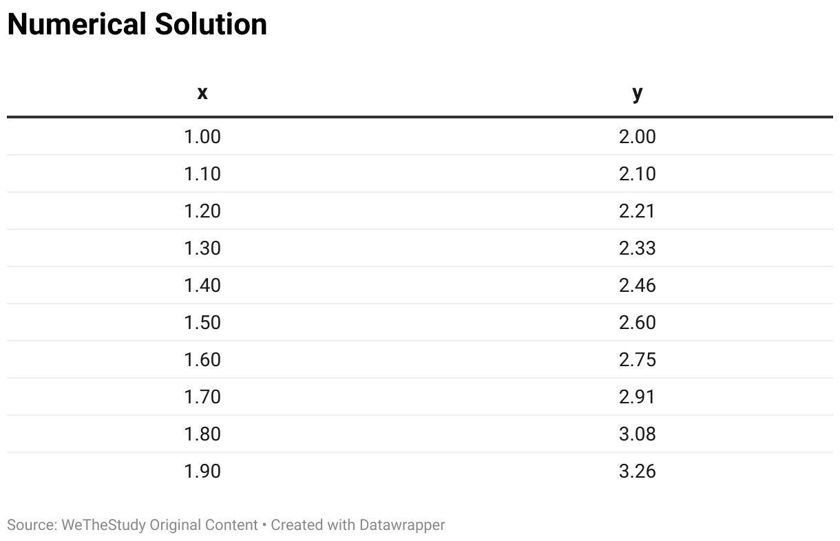
We can plot these values in a graph to show the solution curve of the differential equation. Note that this plot is only an estimate like the graphical approach.
To find the math expression that would fit the points. We can use the table of values and perform a regression analysis. The result will generate an approximate math function.
Summary
Euler's Method is another approximation method of solving differential equations using a table of values.
It is an iterative procedure in which we consider a single coordinate point and solve for successive points along the solution curve using any step value \(\Delta_x\).
The smaller \(\Delta_x\), the better the approximation is.
Equation-wise, it is equal to \(x_{n+1} = x_n + \Delta_x\) and \(y_{n+1} = y_n + y^\prime \cdot \Delta_x\)
We solve for these coordinates, summarize them in a table of values, and plot a curve using these points.


