How to Use Virtual Work to Solve Flexural Deflections?
Let's explore how to compute the deflection of our beam example using the Virtual Work Method. We shall use this to illustrate how to use the method to find the slope and translation at a point.
The first step is to represent each required deflection component with a unit load and assume its direction. For this example, we'll consider the following:
The vertical deflection at \(C\) is downward; hence, the unit load must also be downward.
The rotation at \(C\) is clockwise; the unit couple should also be clockwise.
We apply these unit loadings to each virtual structure, as seen below.
Formulate M, E, I, and m-Equations
The next step is to find the explicitly defined \(M\), \(E\), and \(I\) equations of the superimposed beam and the bending moment equations of our virtual structures \(m_v\) and \(m_{\alpha}\).
For this illustrative problem, we will not yet consider variations in the beam's flexural rigidity \(EI\); hence, we will assume it is constant.
Segment AB
We place a cutting plane between points \(A\) and \(B\) and consider the left section. The \(M\) and \(m\)-equations for this segment \(\left(0 \le x \lt 2 \right)\) are the following:
\(M_{A B}=27\)
\(m_{v_{A B}}=0\)
\(m_{\alpha_{A B}}=0\)
Segment BC
To determine \(M\) and \(m\) for \(BC\) \(\left(2 \le x \lt 6.5 \right)\), we place a section between said points and again investigate the left part:
Next, we consider segment \(CD\) \(\left(6.5 \le x \lt 11 \right)\) and investigate the \(M\) and \(m\) equations for it. Like the previous segments, we place a section between \(C\) and \(D\). We can still choose either the left or right part in formulating the equations (depending on what is convenient). For this instance, we will still use the left section:
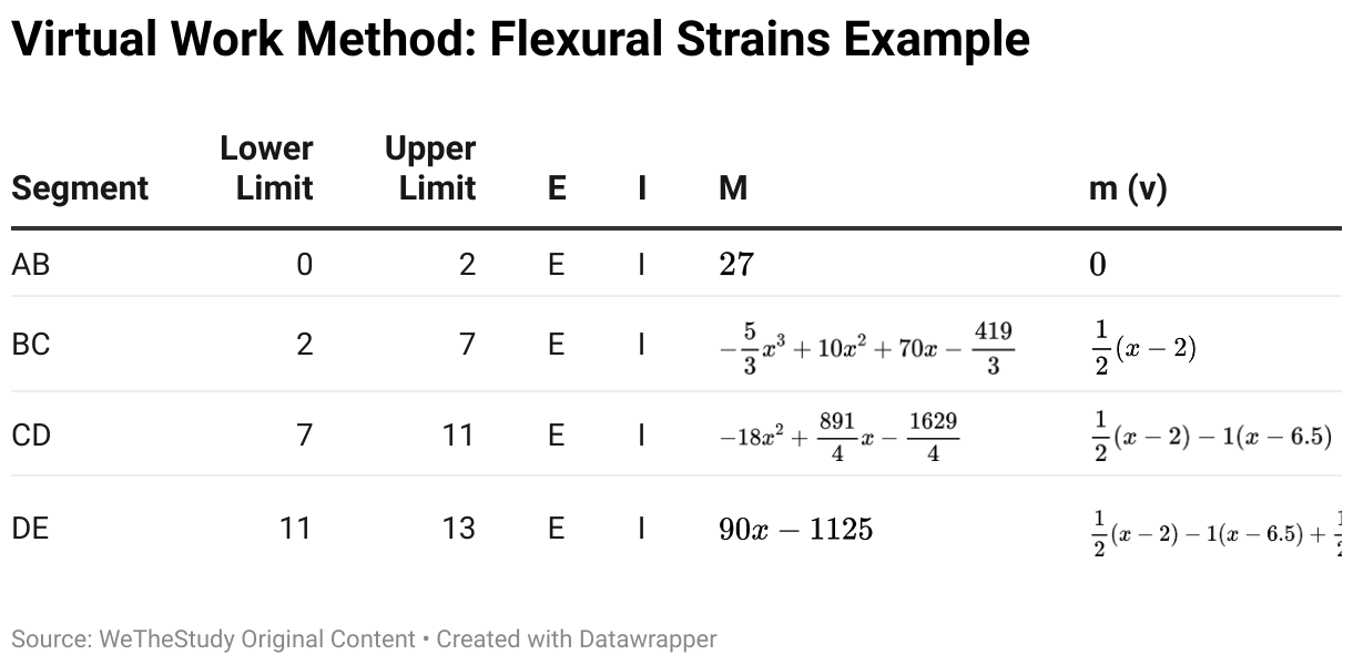
After finding \(M\) and \(m\)-equations for all segments, we can summarise our results using a table.
The summarized table is for the deflection at point \(C\). If we want to find the deflection components at another point, say at \(B\), we need to set up another set of equations and table for it.
Apply Virtual Work Equations
The remaining thing to do is to apply the virtual work equations to solve for \(\Delta_{C_v}\) and \(\theta_C\). Let's begin with the vertical translation at \(C\):
\(1 \times \Delta_{C_v}=\int_{x_1}^{x_2} \frac{M m_v}{E I} d x\)
\(1 \times \Delta_{C_v}=\frac{1}{E I} \int_0^2(27)(0) d x+\frac{1}{E I} \int_2^{6.5}\left(-\frac{5}{3} x^3+10 x^2+70 x-\frac{419}{3}\right)\left[\frac{1}{2}(x-2)\right] d x\)
\(+\frac{1}{E I} \int_{6.5}^{11}\left(-18 x^2+\frac{891}{4} x-\frac{1629}{4}\right)\left[\frac{1}{2}(x-2)-1(x-6.5)\right] d x+\frac{1}{E I} \int_{11}^{12.5}(90 x-1125)\)
\(\left[\frac{1}{2}(x-2)-1(x-6.5)+\frac{1}{2}(x-11)\right] d x\)
\(\Delta_{C_v}=\frac{142155}{64 E I}\)
\(\Delta_{C_v}=\frac{2221.17}{E I}\)
Next, we solve for the rotation at C:
\(1 \times \theta_C=\int_{x_1}^{x_2} \frac{M m_\alpha}{E I} d x\)
\(1 \times \Delta_{C_v}=\frac{1}{E I} \int_0^2(27)(0) d x+\frac{1}{E I} \int_2^{6.5}\left(-\frac{5}{3} x^3+10 x^2+70 x-\frac{419}{3}\right)\left[-\frac{1}{9}(x-2)\right] d x\)
\(+\frac{1}{E I} \int_{6.5}^{11}\left(-18 x^2+\frac{891}{4} x-\frac{1629}{4}\right)\left[-\frac{1}{9}(x-2)+1\right] d x+\frac{1}{E I} \int_{11}^{12.5}(90 x-1125)\)
\(\left[-\frac{1}{9}(x-2)+1+\frac{1}{9}(x-11)\right] d x\)
\(\theta_C=-\frac{1215}{32 E I}\)
\(\theta_C=-\frac{37.97}{E I}\)
With translation and rotation at \(C\) solved, the only thing left to do is to verify our assumptions for directions:
Since the computed vertical translation is positive-sensed, our assumption that point \(C\) moved downward is correct.
On the other hand, rotation at \(C\) is negative, which means that the point rotated counterclockwise instead of clockwise.